In this article, we’ll explore the methods of validating risk models in the context of insurance pricing. For a model to provide meaningful insights, it has to be validated, meaning we need to confirm that it reflects real-world behavior and that its predictions align closely with the data. We’ll focus on two main approaches: visual methods and statistical measures.
When pricing insurance (see our previous post), you usually need to build risk models. A risk model predicts measurable amounts of insurance risk, such as the expected value of claims that may come in on a policy. The two most common are claim frequency and claim severity. Multiply those together, and you get the basis for an insurance premium, often called the actuarial or burning cost. These components can be broken down further by claim type (for example, bodily injury or property damage) or by claim size (such as attritional or large losses).
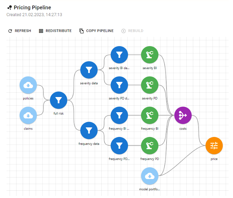
In some cases, combining multiple models produces more accurate results, since each one may capture different patterns in the data. Because these models need large amounts of data to train, they’re best suited for high-volume lines, such as auto, home, or health. Lines with limited data, like life, specialty, or low-volume commercial, often need a different approach.
The most important KPI in insurance is the loss ratio, which represents the amount of claims paid (including claim adjustment expenses) divided by premiums earned. It’s the most widely used measure for assessing the health of a business line.
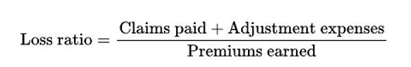
The numerator includes the claim that occurred during a period, while the denominator reflects the expected claim plus expenses. If the premium is calculated accurately, the loss ratio stays stable. But if the expected claims are underestimated, the insurer ends up paying more than planned, leading to a higher loss ratio. That’s why pricing actuaries invest so much time in building accurate risk models and analyzing them in detail.
This raises an important question: how do you know your model isn’t just good, but actually better than earlier versions? And how do you decide which one to use? That’s where different statistical tests and validation techniques come in. Let’s look at some of the most common ones.
Visual methods
The easiest way to understand how well a model performs is to visualize it. Charts and plots make it easy to see where predictions align with reality and where they don’t. Unlike many statistical scores, most visuals don’t need another model for comparison. You can simply see what’s working and what’s not.
Target vs. Predicted
One of the most straightforward charts is the Target (or Actual) vs. Predicted plot.
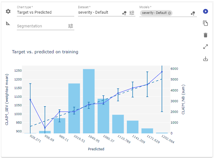
This chart shows how a model’s predictions compare to actual outcomes. It plots the average predicted values against the average target values. In a perfect model, every point would fall neatly along the diagonal reference line. In practice, you just want your line to stay close, especially in the areas with the most data. The bars in the background show frequency, helping you see where the model tends to over- or underestimate, such as when it predicts higher losses than what actually occurred for large claims.
One Way chart
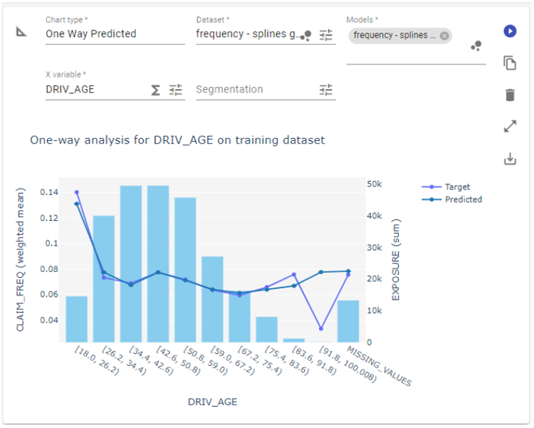
With a One Way chart, you’re looking at two lines: the model’s average prediction and the actual average outcome, plotted against a single variable, like driver age or vehicle type. The bars in the background show how much data you have for each segment. This view helps you understand how the model behaves across your portfolio.
When the two lines start to drift apart, it could mean the model needs further tuning or simply that there’s less data in that range. Charts like this make it easier to spot trends and decide whether to adjust the model, group values differently (binning), or apply a smoothing technique such as splines.
Geo chart
The Geo chart works the same way but uses location instead of numeric variables. It plots predictions and actuals on a map, showing where they line up and where they don’t.
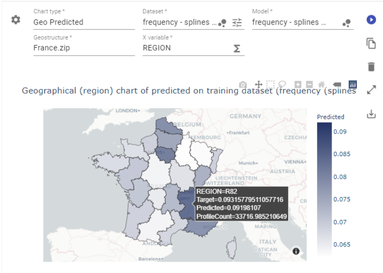
Figure 5. Geo-predicted chart from PricingCenter
The advantage here is clarity. It makes regional differences easy to distinguish. If your model uses geography-based features, like region codes or city names, this chart helps you see where predictions are strong and where they might need smoothing or regrouping.
Lorenz plot
The Lorenz plot is especially useful when you’re working with the Gini index to evaluate a model.
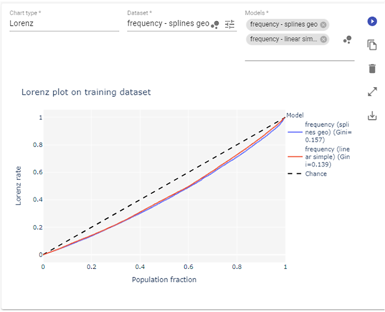
The Gini index is based on the area between the central line and the Lorenz rate line. It shows how well the model captures variation in the target variable and how effectively it distinguishes between different risk profiles.
When the plot line stays close to the central diagonal, it means the model’s output isn’t very correlated with the actual data, and the predictions show little variance. In other words, the model isn’t distinguishing much between different risk profiles. A flat or nearly constant prediction would look like this and would give a Gini value close to zero.As the line bends toward the bottom-right corner, it shows that the model captures more structure in the data, recognizing that some profiles have higher or lower target values. On the other hand, Gini values closer to 1 may indicate overfitting, where the model seems to reflect the data almost perfectly rather than learning from it.
The Lorenz rate represents the percentage of total true values that correspond to predictions not greater than a given prediction level.
There’s an important caveat here, similar to the synthetic Gini score: this information shouldn’t be used on its own. The Lorenz plot is most useful for tracking progress as you refine a model, not for evaluating performance in isolation. On its own, neither the plot nor the Gini score provides actionable insight. But when you compare two or more models trained on the same target variable, the one with the plot line farther from the diagonal generally performs better.
Measures
Which statistical measures should you use to validate a risk model? In addition to visualizations, there’s a wide range of metrics designed to summarize model performance in a single number. Unlike plots, these metrics are synthetic, one-dimensional values, so they simplify a complex picture. That’s why they need to be used carefully: they capture only part of the story.
Below are some of the measures commonly used by actuarial data scientists. Let’s take a closer look at a few of them.
Gini score
Let’s start with the Gini score, which we already touched on in the Lorenz plot section. In data science, this metric isn’t the same as the Gini index used in economics, though the idea is similar.

The score summarizes the information contained in the Lorenz plot and shows how well the model distinguishes target values between different profiles. A single value of the Gini score doesn’t give a complete picture of model fit. We generally aim for values closer to 1, but a score of 1 itself isn’t ideal. It would mean that all values belong to a single profile.
The “ideal” value depends on the model and dataset, so it can’t be defined universally. Instead of focusing on one number, compare Gini scores between variants of the same model. The model with the higher Gini score is considered to be the better one.
AIC and BIC
AIC and BIC stand for Akaike Information Criterion and Bayesian Information Criterion, respectively. Both are used to estimate prediction error and help compare different models. Like the Gini score, they’re most useful for model selection. Each one is based on the model’s likelihood function and the number of parameters it uses.
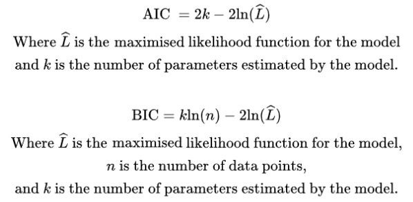
In simple terms, AIC and BIC show how much information is lost when a model tries to represent the real process. The higher the value, the more information is lost and the lower the model quality. Both are influenced by sample size and include penalty terms for model complexity. That means larger datasets and models with more parameters tend to produce higher values.
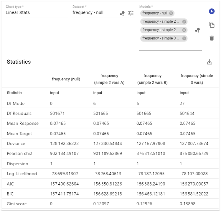
So how do you use AIC and BIC correctly? Imagine you have two versions of the same model (for example, a claim frequency model) trained on the same dataset. The model with the lower AIC or BIC value is generally more robust and should be considered the better one.
Looking at the table above, all four models were trained on the same data. AIC identifies the last one (“simple 3 vars” with three variables) as the best, while BIC favors the third (“simple 2 vars B,” a variant of the two-variable model). The second and third models have the same number of parameters, so in that case, comparing them with AIC/BIC is the same as comparing their log-likelihoods.
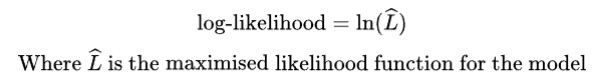
Log-likelihood
This statistic is closely related to AIC/BIC, as it serves as the basis for how they’re calculated. Unlike AIC and BIC, it doesn’t include any penalty terms, so it can be applied more broadly. However, it must always be used with the same dataset, since its value depends on the sample.
When comparing models, higher values are better. Simply treat them as regular numeric comparisons. This measure also allows for a likelihood-ratio test of goodness of fit. The only requirement is that the models are nested, meaning the simpler model is a constrained version of the more complex one.
Dispersion
In GLM or GAM frameworks, some distributions require a dispersion parameter to adjust the variance. Ideally, this value should be close to 1, as shown in the earlier examples. But sometimes, the model’s variance doesn’t line up with what’s in the data. In those cases, the dispersion parameter helps fine-tune the fit, adjusting the model so it better reflects the observed variance. Essentially, it shows the scale of that mismatch between the model and the data.
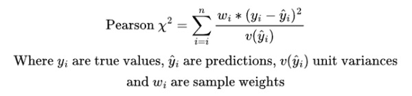
Pearson chi-squared
The Pearson chi-squared value is the test statistic used in the goodness-of-fit test based on the chi-squared distribution. Its value should be compared to the critical values for the corresponding number of degrees of freedom to assess the model’s fit.
Deviance
In the process of model fitting, predictions are evaluated against the data using an appropriate unit deviance function. Each distribution family has a natural choice for this function.
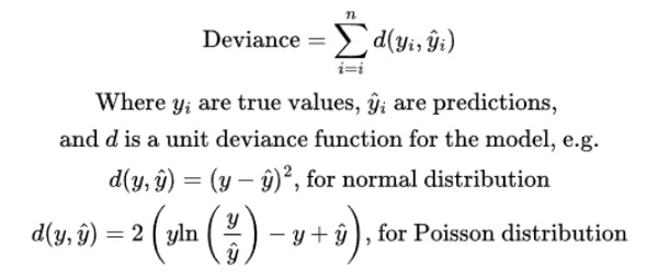
The measure shown on the chart represents the total amount of unit deviances for the entire dataset. It tells us, in aggregate, how far the model’s predictions are from the true values. Like AIC and BIC, this measure depends on sample size, so it can only be used to compare models fitted with the same distribution family and trained on the same dataset.
The number alone doesn’t provide much information, but it can be used to select the better-fitted model.
The statistics above apply to linear models and are always available within the linear model design of the PricingCenter platform. However, for models in general, including non-linear and machine learning models, other measures are also commonly used. The most frequent ones are MAE (Mean Absolute Error), MSE (Mean Squared Error), and RMSE (Root Mean Squared Error).
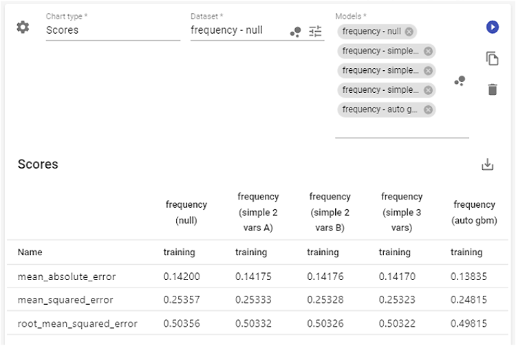
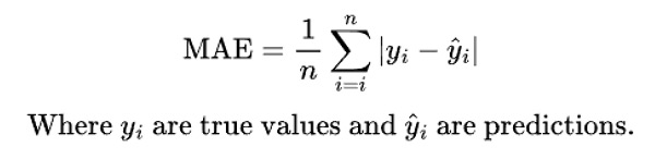
Mean absolute error
This measure calculates the average of the absolute differences between the target and predicted values. It shows, on average, how far the model’s predictions are from the actual data. Naturally, it’s always non-negative, and a value of zero would mean the model predicts the data perfectly. Higher values, on the other hand, suggest the model fits the data less accurately.
What’s considered a “good” MAE depends on the problem. For example, if we’re estimating claim frequency per policy (usually a small positive number below 1) and the model is trained on exposure-adjusted claim count data, most records will have a value of 0, and only a few will be above 1. In such cases, it’s impossible to achieve a very low MAE, because for most data points, the absolute difference essentially equals the prediction value.
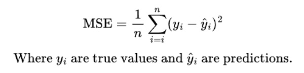
Mean squared error (MSE)
The idea behind MSE is similar to MAE, but instead of taking the absolute value of the difference, it squares the differences before averaging them. This means MSE penalizes larger errors more heavily than smaller ones. When the model’s predictions diverge significantly from the data, the MSE increases sharply. When the predictions are close, the impact on MSE is much smaller.
In the example above, the MSE is higher than the MAE, which shows that the larger positive deviations in claim counts are more pronounced in this metric.
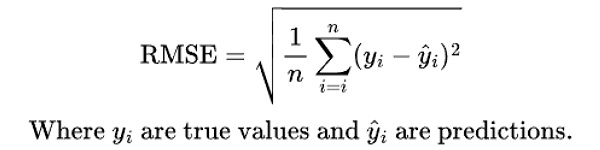
Root mean squared error (RMSE)
RMSE is directly related to MSE—it’s simply the square root of the MSE score. Taking the square root brings the value back to the same range as the original predictions, making it easier to interpret. This helps relate the result to the actual scale of the target variable, which isn’t possible with MSE alone.
Now what?
We’ve now covered the basics of risk modeling in insurance pricing, including what a risk model is, how it relates to premiums, and why accuracy matters. The quality of a risk model is directly reflected in the difference between a company’s actual loss ratio and its expected value.
That’s why it’s so important to evaluate model quality carefully, using both statistical measures and visual methods. Some of the techniques discussed above can be applied to any type of model—linear, non-linear, or machine learning, while others are specific to linear models. Together, they give you the tools to identify, compare, and refine models so you can select the one that performs best.
Key takeaways
- Charts help you visually assess how well the model fits the data—and the more complex the model, the more charts you’ll need to validate it. This ensures no major discrepancies go unnoticed.
- Statistical measures are useful for comparing different versions of the same model. These values don’t exist in isolation; they only have meaning when compared across models trained on the same dataset.
- Use these metrics to guide decisions when refining your model. For example, deciding how to treat a variable or whether adding a new risk factor improves the fit.
Next steps
We haven’t yet touched on methods created specifically to explain machine learning models. You might already be familiar with some of them, like the ceteris paribus (single-profile) plot or partial dependency (average-response) plot. We’ll explore those in more detail later, as they’re key to understanding how complex models make predictions.
With the concepts and techniques covered so far, you’re now better equipped to develop, evaluate, and validate high-quality risk models. And if you’re interested in software that helps you not only calculate but also evaluate, validate, and visualize your models, PricingCenter is built for exactly that.